Computational Fluid Dynamics (CFD): Difference between revisions
Rmanwaring (talk | contribs) No edit summary |
No edit summary |
||
| (2 intermediate revisions by 2 users not shown) | |||
| Line 6: | Line 6: | ||
|- | |- | ||
|style="text-align:center; font-size:90%;"| Analysis of spillway [[hydraulics]] using Computational Fluid Dynamics (CFD). | |style="text-align:center; font-size:90%;"| Analysis of spillway [[hydraulics]] using Computational Fluid Dynamics (CFD). | ||
(Image Source: Gannett Fleming) | |||
|} | |} | ||
<!-- Delete any sections that are not necessary to your topic. Add pictures/sections as needed --> | <!-- Delete any sections that are not necessary to your topic. Add pictures/sections as needed --> | ||
Computational fluid dynamics utilizes applied mathematics and physics to calculate the flow field throughout a flow domain defined by appropriate boundary conditions. Once the entire flow domain is partitioned into a grid of appropriately-sized computational cells, the Navier-Stokes equations, in conjunction with equations for each conservation law (mass, momentum, and energy), are solved in each grid cell throughout the flow domain | Computational fluid dynamics utilizes applied mathematics and physics to calculate the flow field throughout a flow domain defined by appropriate boundary conditions. Once the entire flow domain is partitioned into a grid of appropriately-sized computational cells, the Navier-Stokes equations, in conjunction with equations for each conservation law (mass, momentum, and energy), are solved in each grid cell throughout the flow domain. The finite volume method and linearized approximations of the partial differential flow equations are employed to solve the Navier-Stokes equations in each grid cell throughout the flow domain. | ||
One of the major challenges in CFD has been, and continues to be, the accurate modeling of turbulence | One of the major challenges in CFD has been, and continues to be, the accurate modeling of turbulence; numerically represented by instantaneously fluctuating flow quantities throughout the flow domain, known as the Navier-Stokes Closure Problem. Several different turbulence models have been developed in an attempt to estimate the instantaneously fluctuating turbulent flow quantities including the use of the Boussinesq Approximation in the use of Eddy Viscosity models, and the Smagorinsky model and sub-grid scale eddy viscosity in Large Eddy Simulation models. The selection of an appropriate turbulence modeling scheme is dependent upon the situation including available computational resources, available time to solve the flow domain, complexity of the flow domain geometry, and desired predictive accuracy of the model. | ||
The major | The major benefits of numerical modeling include the elimination of the space, time, and resources required to build and house a physical model; the elimination of the need to apply scaling factors; the flexibility to make significant changes to flow domain geometries; and the ability to quantify, collect, and visualize all flow quantities including pressures, velocities, air concentrations, etc. throughout the entire flow domain. | ||
<!-- For information on notation for in text citations visit https://www.mediawiki.org/wiki/Help:Cite Or simply enclose the citation as shown <ref> citation </ref> in the location of the in text mention. Citations will automatically populate below--> | <!-- For information on notation for in text citations visit https://www.mediawiki.org/wiki/Help:Cite Or simply enclose the citation as shown <ref> citation </ref> in the location of the in text mention. Citations will automatically populate below--> | ||
Latest revision as of 21:27, 28 March 2024

|
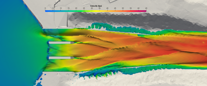
| Analysis of spillway hydraulics using Computational Fluid Dynamics (CFD).
(Image Source: Gannett Fleming) |
Computational fluid dynamics utilizes applied mathematics and physics to calculate the flow field throughout a flow domain defined by appropriate boundary conditions. Once the entire flow domain is partitioned into a grid of appropriately-sized computational cells, the Navier-Stokes equations, in conjunction with equations for each conservation law (mass, momentum, and energy), are solved in each grid cell throughout the flow domain. The finite volume method and linearized approximations of the partial differential flow equations are employed to solve the Navier-Stokes equations in each grid cell throughout the flow domain.
One of the major challenges in CFD has been, and continues to be, the accurate modeling of turbulence; numerically represented by instantaneously fluctuating flow quantities throughout the flow domain, known as the Navier-Stokes Closure Problem. Several different turbulence models have been developed in an attempt to estimate the instantaneously fluctuating turbulent flow quantities including the use of the Boussinesq Approximation in the use of Eddy Viscosity models, and the Smagorinsky model and sub-grid scale eddy viscosity in Large Eddy Simulation models. The selection of an appropriate turbulence modeling scheme is dependent upon the situation including available computational resources, available time to solve the flow domain, complexity of the flow domain geometry, and desired predictive accuracy of the model.
The major benefits of numerical modeling include the elimination of the space, time, and resources required to build and house a physical model; the elimination of the need to apply scaling factors; the flexibility to make significant changes to flow domain geometries; and the ability to quantify, collect, and visualize all flow quantities including pressures, velocities, air concentrations, etc. throughout the entire flow domain.
Citations:
Revision ID: 7840
Revision Date: 03/28/2024
